
When the number of observations in one class is much more than the other, it is difficult to train a vanilla CNN classifier. The CNN classifier may consider that all observations are from the main class to achieve high accuracy.
One way to handle this problem is by using oversampling or downsampling to make data balanced. Also, adjusting class weights to force the classifier to handle data in the rare class is also a great idea.
However, using the above methods may sometimes cause model overfitting when data is extremely imbalanced. Therefore, we’ll look at another method, which is called anomaly detection, to deal with this case.
We will assume the observations in the main class as normal data, and use only these data to train our model. Then, we are able to predict whether a new observation is normal. You might ask how to detect abnormal data when the model didn’t train on these data. The following is a simple example to show how anomaly detection work.
— Implementation —
We can use Keras and Scikit Learn to implement anomaly detection within a few lines of code.
First, import libraries to build the model. These four libraries are all we need.
Second, we can use pre-trained models as feature representations to transform images into a better feature space.
We use Keras to get a VGG16 model pre-trained on ImageNet and get the output of the chosen layer. Then, we pass the output through a global average pooling layer to reduce dimensions.
To implement one class classifier, we use a clustering model, Gaussian mixture model (GMM), from Scikit Learn. So, build a GMM with one component.
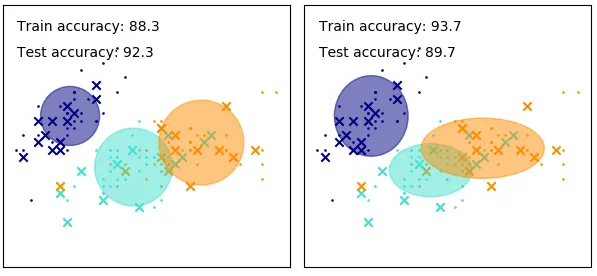
As shown in Figure 2., the data closer to the center of a Gaussian distribution are more likely to be normal. By choosing the range of the distribution, we are able to determine whether the observation is normal or not.
It’s time to import a dataset to see how the model works. We use MNIST dataset from Keras. We assume ‘1’ as normal data and ‘7’ as abnormal data. Thus, we only use ‘1’ as training data and use both ‘1’ and ‘7’ as test data.
reshape_x: according to Keras’s VGG pre-trained model, the minimum size of images is 30 * 30, so we have to resize our images and transform them into 3-channel images.
There are merely two lines to train our model. First, use the VGG model to extract features from training data. Then, use the results as the GMM’s input data to it.
— Result —
Using GMM’s score_samples function, we can easily compute the likelihood of data. Assuming threshold as the mean likelihood of training data plus 3 times the standard deviation, we can predict our testing data.
We use the VGG model to extract features from testing data. Then, we use the trained GMM to compute the likelihood of results. Finally, we can detect anomaly if the observation’s likelihood is smaller than the threshold.

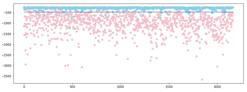
Let’s visualize our results! We draw scattergram, and the x-axis is the index of data and the y-axis is the score. We plot ‘1’ as blue points and ’7’ as pink points and plot the threshold as the black line. We can see that most of the points can be separated by the threshold. That’s how we detect abnormal data.
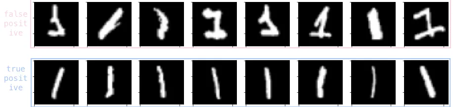
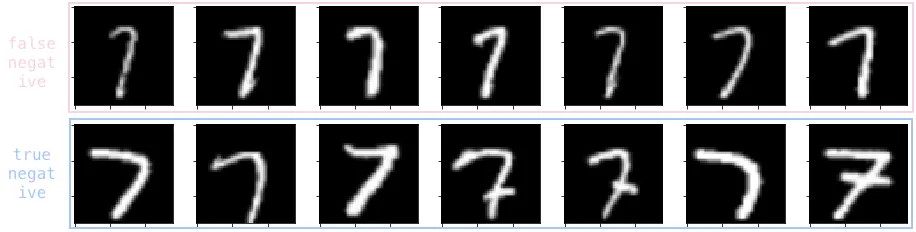
We can also check the failure cases. The figure below shows that the model is more likely to make mistakes when ‘1’ is more complicated and when ‘7’ is too thin.
To get better accuracy, we can replace the pre-trained model by an autoencoder to get better feature representations. Although models pre-trained on ImageNet can extract great features from images, the images in MNIST is pretty different from images in ImageNet. We may get a worse result if we use a dataset which is much different from ImageNet. Besides, there are lots of ways to implement anomaly detection, feel free to try another one.
— Reference—
[1] ICML 2018 Paper Deep One-Class Classification